Scraping Pro Football Reference
Introduction
As an avid sports fan and data scientist, I’ve always liked looking into the statistics behind sports. And given the very public nature of NFL games and their corresponding box scores and statistics, I was quite surprised that I wasn’t easily able to track down a good dataset for the NFL statistics that I was interested in. Specifically, I was looking for career statistics for all players, past and present, in the NFL. I knew the data was out there and had been organized by various websites, most notably Pro Football Reference, but I couldn’t seem to find anything that matched exactly what I wanted. The closest I found was a dataset, seen here, from Zack Thoutt. However, it was 7 years out of date, lacked all the columns I wanted, and the scraper found on his github profile no longer works due to some changes to how the PFR website handles its tables.
So, I decided to write a simple web scraper for PFR that would get me the data I wanted. The code for the web scraper and the resulting data can be found at this github repo. Big shoutout to Zach Thoutt for his original scraper, seen here, as I referenced it to get the foundation of my scraper.
In this blog post, I’m going to go over the resulting data from the scraper, clean it up a bit, and show some simple analysis and visualizations as examples of uses of the dataset.
Importing and Cleaning the Dataset
import numpy as np
import pandas as pd
import seaborn as sns

player_stats = pd.read_csv('player_stats.csv')
Given the often tenuous nature of web scraping, the data is likely to contain some missing values. This code tells me how many missing values each column has.
player_stats.isnull().sum().loc[player_stats.isnull().sum() > 0]

# Code Output
position 10
height 259
weight 259
dtype: int64
I can see that we have 3 columns with missing values, position, height, and weight. I plan on doing analysis later using position, and it only has 10 missing values, so let’s see if I can fix these values. First, I want to take a look at the effected rows.
missing_position = player_stats[player_stats['position'].isnull()]
missing_position.iloc[:, :9]
| player_id | name | position | career_begin | career_end | active | height | weight | games_reg | |
|---|---|---|---|---|---|---|---|---|---|
| 661 | 662 | Daniel Archibong | nan | 2021 | 2021 | False | 6-6 | 300lb | 2 |
| 2766 | 2767 | Josiah Bronson | nan | 2021 | 2022 | False | 6-3 | 295lb | 8 |
| 5229 | 5230 | Tyler Coyle | nan | 2021 | 2022 | False | 6-1 | 210lb | 3 |
| 5403 | 5404 | Tae Crowder | nan | 2020 | 2023 | True | 6-3 | 235lb | 43 |
| 5865 | 5866 | Michael Davis | nan | 2017 | 2024 | True | 6-2 | 196lb | 122 |
| 10062 | 10063 | JaQuan Hardy | nan | 2021 | 2021 | False | 5-10 | 225lb | 3 |
| 10797 | 10798 | Grant Hermanns | nan | 2022 | 2022 | False | 6-7 | 305lb | 2 |
| 16258 | 16259 | Nate McCrary | nan | 2021 | 2021 | False | 6-0 | 213lb | 1 |
| 21560 | 21561 | Lenny Sachs | nan | 1920 | 1926 | False | nan | nan | 0 |
| 22884 | 22885 | Chris Smith | nan | 2024 | 2024 | True | 6-1 | 305lb | 5 |
Looking at all the players that are missing their position, there doesn’t seem to be any pattern as to why it’s missing. It is mostly players from recent years, but there is a player from the 1920’s. There’s a mix of active and non-active players, some players have played quite a few games while others only played a couple, and only one of the ten is also missing their height and weight. Looking at the first player, Daniel Archibong, his personal Pro Football Reference page, seen here, shows that he was listed as a DT for the 2 games he played in Pittsburgh back in 2021. For some reason, his position isn’t listed in the parentheses following his name on the “Football Players with Last Names Starting with A” page, seen here. That’s why his position was not recorded by the scraper. Regardless, it is clear that Daniel Archibong was a DT, so his position can be updated as such. Given there are only 9 other players with missing positions, they can similarly be solved manually. All I have to do is update each of their positions with the following code:
player_stats.loc[player_stats['player_id'] == 662, 'position'] = 'DT'
player_stats.loc[player_stats['player_id'] == 2767, 'position'] = 'DT'
player_stats.loc[player_stats['player_id'] == 5230, 'position'] = 'S'
player_stats.loc[player_stats['player_id'] == 5404, 'position'] = 'LB'
player_stats.loc[player_stats['player_id'] == 5866, 'position'] = 'CB'
player_stats.loc[player_stats['player_id'] == 10063, 'position'] = 'RB'
player_stats.loc[player_stats['player_id'] == 10798, 'position'] = 'G'
player_stats.loc[player_stats['player_id'] == 16259, 'position'] = 'RB'
player_stats.loc[player_stats['player_id'] == 21561, 'position'] = 'LE'
player_stats.loc[player_stats['player_id'] == 22885, 'position'] = 'DL'
Now, I can quickly verify that there are no longer any missing values in position.
player_stats['position'].isnull().sum()

# Code Output
0
As for height and weight, each column is missing 259 values. I scraped both columns together with a single regex expression, which gives me the sense that all the missing values for these columns come from pages where my regex failed to find a match. This would mean that all the missing values for both columns are in the same 259 rows. I’m going to take a peek at the first 10 rows that are missing height to double check.
missing_height = player_stats[player_stats['height'].isnull()]
missing_height.iloc[:10, :9]
| player_id | name | position | career_begin | career_end | active | height | weight | games_reg | |
|---|---|---|---|---|---|---|---|---|---|
| 460 | 461 | Anderson | WB | 1922 | 1922 | False | nan | nan | 1 |
| 582 | 583 | Jaby Andrews | WB-DB | 1934 | 1934 | False | nan | nan | 2 |
| 782 | 783 | Burl Atcheson | E | 1922 | 1922 | False | nan | nan | 1 |
| 923 | 924 | Backnor | C | 1921 | 1921 | False | nan | nan | 1 |
| 1103 | 1104 | Hugh Bancroft | E | 1923 | 1923 | False | nan | nan | 2 |
| 1283 | 1284 | Eddie Barnikow | FB | 1926 | 1926 | False | nan | nan | 2 |
| 1326 | 1327 | John Barsha | FB | 1920 | 1920 | False | nan | nan | 3 |
| 1485 | 1486 | Fred Beach | G | 1926 | 1926 | False | nan | nan | 1 |
| 1564 | 1565 | John Beckwith | HB | 1920 | 1920 | False | nan | nan | 3 |
| 1776 | 1777 | Eddie Benz | E | 1922 | 1922 | False | nan | nan | 1 |
It certainly seems to be the case that every row that is missing height is also missing weight. This next code snippet can confirm this.
missing_height_and_weight = missing_height['player_id'] == player_stats[player_stats['weight'].isnull()]['player_id']
print(missing_height_and_weight.unique())

# Code Output
[ True]
Let’s look a little further into this to see if this is a problem with my scraper or a problem with the underlying data. One strange thing I immediately notice is in the first row. The player has only one name, “Anderson”, and played a single game in 1922. Their individual Pro Football Reference page, seen here, shows very little data, only that they played in one game. No full name, no statistics, no height or weight. It seems the scraper did all it could here as this page offers little value, and it should probably be removed from the data set. We can see what looks like a similar case in the fourth row, a played named only “Backnor” with one career game in the 1920’s as well. This looks like an unrelated problem, so let’s revisit this after we solve the height and weight situation.
Moving on to the second row, on Jaby Andrew’s PFR page, seen here, Jaby Andrews has a listed weight of 208lbs, but no listed height. However, the data shows both Jaby’s height and weight as missing, instead of just the height. This is because the scraper is expecting to find a height and weight regex match in the form of “X-Y, Zlb”, where X, Y, and Z are numbers. When a page is missing the height, like Jaby Andrew’s, or weight, the regex entirely fails to find a match, leaving both height and weight as NaN. So this is clearly an issue with the scraper. I could solve this rather easily by performing two separate regex matches to find height and weight independently. This would give us more complete data, but each of these 259 rows would still be missing either height or weight. So in this case, I’m going to choose to just drop all 259 columns to completely remove all missing values from the data. 1
player_stats = player_stats.dropna(subset=['height', 'weight'])
Now we can revisit the earlier issue of rows with players like “Anderson” and “Backnor”. While those two specific instances were removed due to their missing height and weight, there will likely be more rows with a similar problem. It seems to me that the easiest way to find all instances of this problem would be to split the name column on every space, which will give us a list, then take the length of each list that results from the split. Any players whose name list is of length 1 is likely a problem.
player_stats['name_list_len'] = player_stats['name'].apply(lambda x: len(x.split()))
one_name = player_stats[player_stats['name_list_len'] == 1]
one_name.iloc[:10, :9]
| player_id | name | position | career_begin | career_end | active | height | weight | games_reg | |
|---|---|---|---|---|---|---|---|---|---|
| 3166 | 3167 | Brunswick | G | 1920 | 1920 | False | 5-10 | 182lb | 1 |
| 20823 | 20824 | Riley | G | 1924 | 1924 | False | 5-11 | 195lb | 1 |
Ah, another pair of players from the 1920’s who only played a single game apiece. I’m going to go ahead and drop these rows from the dataset as well.
A side note here is that the player_id I assigned to each player is simply their location in a list of all player names sorted alphabetically, where the first player has player_id = 1. I chose to start at 1 to avoid any player having a player_id of 0. However, when pandas gives indices to the rows in DataFrames, their indexing starts at 0. So “Brunswick” has a player_id of 3167, while their index in the DataFrame is 3166. This can cause off-by-one errors if not careful. I find it to typically not be an issue as long as I remembered to use the DataFrame indices when referring to specific rows, such as when dropping rows or using iloc.
player_stats.drop(3166, inplace=True)
player_stats.drop(20823, inplace=True)

print('DataFrame dimensions: ' + str(player_stats.shape))
print('Number of missing values: ' + str(player_stats.isna().sum().sum()))

# Code Output
DataFrame dimensions: (27695, 163)
Number of missing values: 0
After cleaning the missing values and rows with only a single name from the data, the DataFrame contains 27695 rows and 163 columns.
Adding Additional Columns
I’m going to create some helper columns to make future analysis easier. The first one is going to be career_length, which will be the number of years the player has played in the league. The equation for this is career_length = career_end - career_start + 1. Adding the one is necessary to correct the off-by-one error. A player whose first year and last year in the NFL were both 2013 played one year, 2013, even though the difference between their first and last year is zero.
player_stats['career_length'] = player_stats['career_end'] - player_stats['career_begin'] + 1
The other column will be position_list. The current position column contains a string with the player’s position. This works great for players with only one listed position. However, for players with multiple listed positions, it contains each position separated by a hyphen in a single string, e.g. "DB-WR" for Deion Sanders. Performing a simple match for all players whose position == “QB” would exclude any players who have any other positions listed, even though they shouldn’t be. So I can just add a new column that splits the string in position on each hyphen and stores the resulting list. 2
player_stats['position_list'] = player_stats['position'].str.split('-')
Exploratory Data Analysis / Visualizations
With all of that done, now it’s quite trivial to perform quick exploratory data analysis on the data from the web scraper. Let’s say I want to see the average number of regular season games played by QBs across all of NFL history, and create a histogram to visualize that data. We can start by filtering the player data to only that of the players where at least one of their listed positions is “QB”.
qb_stats = player_stats[player_stats['position_list'].apply(lambda x: 'QB' in x)]
print(str(qb_stats.shape[0]) + ' QBs in the dataset')

# Code Output
1087 QBs in the dataset
We are left with 1087 players listed as a quarterback across all of NFL history. From here, it is easy to find summary statistics about regular season games played. And, using the python graphical package of your choice (in my case, seaborn), it’s very easy to quickly make visualizations, like histograms or scatterplots.
print(qb_stats['games_reg'].describe())
sns.histplot(qb_stats, x='games_reg', binwidth=10).set(title='Regular Season Games Played (QBs)')

# Code Output
count 1087.000000
mean 46.971481
std 57.329426
min 0.000000
25% 6.000000
50% 22.000000
75% 71.500000
max 340.000000
Name: games_reg, dtype: float64
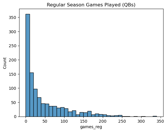
The summary statistics show the mean number of regular season games played is 46.97, but the standard deviation, at 57.33, is huge relative to the mean, due to the large right skew seen in the histogram. The median of 22 is a better measure of central tendency when looking at the histogram. The histogram also illustrates that most quarterbacks appear in 10 regular season games or fewer, and as the number of career games increases, there are fewer and fewer QBs whose career spanned that many regular season games. This difference in games played causes most charts of counting statistics to look similar to the above chart, with a large bar in the start then a shrinking tail skewed right. More games means more opportunity to rack up numbers. For instance, let’s look at the histogram of career regular season passing yards.
sns.histplot(qb_stats, x='pass_yds_reg', binwidth=1000).set(title='QB Career Regular Season Passing Yards')
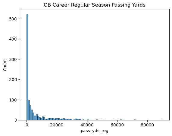
Due to the correlation between regular season games played and passing yards, the same trend appears in the chart, only even more exaggerated. Of the 1087 quarterbacks we started with, the chart shows that over 500 of them, or about half, never eclipse 1000 career regular season passing yards. While it’s hard to play a lot of games in the league as a quarterback, it seems to be even harder to rack up many thousands of passing yards. We can calculate the numerical correlation between career length and regular season passing yards, then use a scatterplot to visualize the relationship between both variables.
print(qb_stats['games_reg'].corr(qb_stats['pass_yds_reg']))
sns.scatterplot(qb_stats, x='games_reg', y='pass_yds_reg')

# Code Output
0.8869475559344511
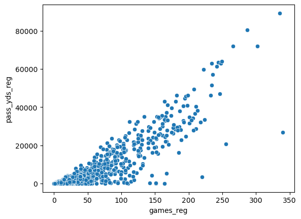
These variables are strongly correlated, with an r value of about 0.88, and the scatterplot visually confirms this. However, this same trend doesn’t appear in histograms for statistics that are rates, such as completion percentage. Below is the corresponding histogram for regular season completion percentage.
sns.histplot(qb_stats, x='pass_cmp_pct_reg').set(title='QB Career Regular Season Completion Percentage')
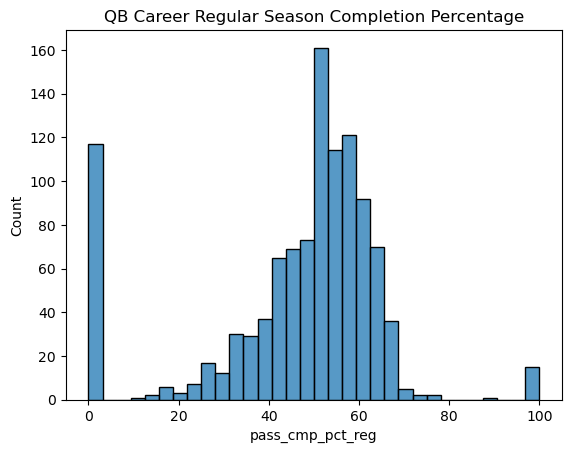
Here see something much closer to a normal curve, with some outliers at both 0 and 100 percent for QBs that have very few passing attempts. Let’s see how different the chart looks if we institue a minimum number of passing attempts to appear on the chart. This is a common way to remove outliers in sports statistics. Pro Football Reference uses a minimum number of 1500 passing attempts to determine career leaders in passing completion, so I will use that as the cutoff.
sns.histplot(qb_stats[qb_stats['pass_att_reg'] >= 1500], x='pass_cmp_pct_reg', binwidth=1).set(title='QB Regular Season Completion Percentage (min. 1500 attempts)')
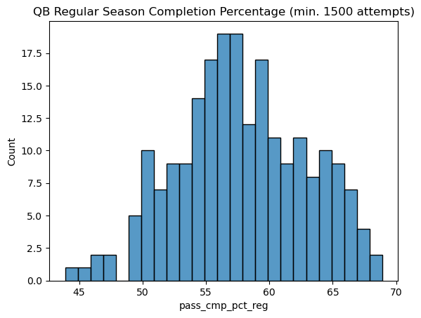
This step completely removes the outliers and shows a more representative picture of quarterback completion percentages.
Conclusion
Hopefully, this has helped illustrate the usefulness of the web scraper and dataset. I was able to extract a dataset of NFL career player statistics, clean it, and perform some basic exploratory data analysis. This dataset is useful for many types of sports analysis, whether it’s analyzing league-wide trends over time, crafting interesting visualizations, or even just creating sports trivia questions.
There is definitely room for the scraper and dataset to improve and grow, most obviously by scraping individual player seasons instead of career statistics. That additional level of granularity would open the door to analysis by age and comparing active players’ career trajectory to retired players, as well as team and season specific analysis that is currently not possible with the current dataset.
If you find this type of sports data science writing interesting, please keep checking in on the blog. One of my goals for 2025 is to regularly post interesting sports analytics stuff here. Also, if you have a github account and think the web scraper is cool or useful, feel free to drop a star on the repo. I really appreciate anyone who hasen taken the time to read all of this, thank you!
-
I’m also partially motivated to not update the scraper right this second due to the fact that the web scraping rate limit on PFR means that fully rerunning the scraper would take about 48 hours, and I do plan on finishing this blog post well before 48 hours from now. ↩
-
It’s technically stored in a pandas Series object, which behaves similarly to, but not exactly like, a base python list. In this situation, they are interchangeable. ↩